
Nick Peterson and Justin Risch have begun to study Big Data, Spark, Hadoop, and the technologies that permeate that environment. This is both a recount of their first experiences working with these technologies, as well as an example to help define the process for those looking to learn Big Data themselves.
Data Gathering
Since we needed both a huge amount of data and data over the course of months, we decided to turn to an unlikely source -- https://www.reddit.com/r/pokemongodev/. When asked, the developers there were more than happy to share their data. After all, with Big Data practices, we might be able to reverse engineer the Pokemon GO spawn algorithm and even predict future events. Forums for data hobbyists -- such as developer forums on reddit or elsewhere -- are often a very valuable resource for people looking to learn Big Data, as the first step is obtaining data!
Data Cleansing
Once we obtained the data, the first step was to get it in a more readable format. It was delivered to us in a .sql file -- great if we were running an SQL Server, but not so much in a HDFS-based system. First step, then, was to remove file headers and commands (such as "insert into table 'pokemon'"), leaving nothing but data in the file. After that, we removed all quotation marks, allowing us to handle the data as more than just strings, especially since the most important data to us was longitude and latitude: not a String, but a pair of Doubles.
First Attempts at Visualization
In an effort to gain a simplistic visualization of the data, Justin decided to print out the coordinates to a bmp file, gaining what was effectively a map of the world if you only saw the world through Pokemon GO's eyes. Here we can see a map of the United States. Blue is a single spawn, while green is two in that area. Yellow is 3, and red is 4 or more.
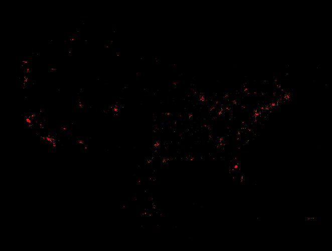
Immediately, we can see a correlation with cell phone coverage (below). This makes sense, as it's a game played on cell phones, but it also confirms a suspicion that players had: The more cell-phone users in an area, the more Pokemon spawn. To be clear, it's not that the cell phone signal spawns Pokemon, but rather that phone companies invest in their infrastructure in areas where there are more smartphone users, and Pokemon spawn where there are more cell phone users.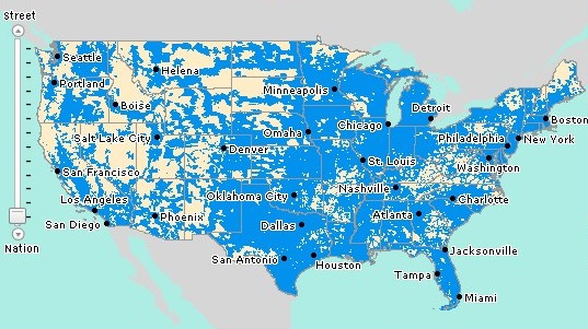
Beyond that simple visualization, we needed to start crunching the numbers to find the information we cared most about -- what was rare, where could it be found, and why there of all places?
Data Analysis
With the data in a much more usable .csv format, Nick decided to use this to do some practice in Spark. It was a fairly simple Spark class written in Scala using the Eclipse Scala IDE, which was used to interpret the data.object MostSpawnedPokemon {
def loadNames() : Map[Int, String] = {
var pokemonNames:Map[Int, String] = Map()
val lines = Source.fromFile("../Data/pokemon.csv").getLines()
for (line <- lines) {
var fields = line.split(',')
if (fields.length > 1) {
pokemonNames += (fields(0).toInt -> fields(1))
}
}
return pokemonNames
}
def main(args: Array[String]) {
// Set the log level to only print errors
Logger.getLogger("org").setLevel(Level.ERROR)
// Create a SparkContext using every core of the local machine
val sc = new SparkContext("local[*]", "MostSpawnedPokemon")
// Create a broadcast variable of our ID -> Pokemon Name map
var nameDict = sc.broadcast(loadNames)
// Read in each Spawn line
val lines = sc.textFile("../Data/AllData.csv")
// Map to (spawnedPokemonId, 1) tuples
val spawned = lines.map(x => (x.split(",")(2).toInt, 1))
// Count up all the 1's for each Pokemon
val spawnedCounts = spawned.reduceByKey( (x, y) => x + y )
// Flip (spawnedPokemonId, count) to (count, spawnedPokemonId)
val flipped = spawnedCounts.map( x => (x._2, x._1) )
// Sort
val sortedCount = flipped.sortByKey()
// Fold in the Pokemon names from the broadcast variable
val sortedCountWithNames = sortedCount.map( x => (nameDict.value(x._2), x._1) )
// Collect and print results
val results = sortedCountWithNames.collect()
results.foreach(println)
}
}
Nick walks through each step of his code in the comments. This ended up being a simple yet solid example of using Broadcast Variables in Spark. Broadcast variables allow the programmer to keep a read-only variable cached on each machine rather than shipping a copy of it with tasks. The output from this was the Pokemon's name and the number of spawn occurrences. Here is a snippet from the output showing the most uncommon Pokemon:
- (machamp,8)
- (kabutops,14)
- (charizard,14)
- (farfetchd,14)
- (muk,15)
- (gyarados,20)
- (raichu,23)
- (omastar,25)
- (alakazam,27)
- (ninetales,27)
This is a fun dataset to work, with and I am going to continue using it as I begin learning more advanced Spark programming. This simple bit of information regarding the rarity of Pokemon ended up helping Justin in some work he did visualizing the data.
Revisualizing with a better understanding of the data
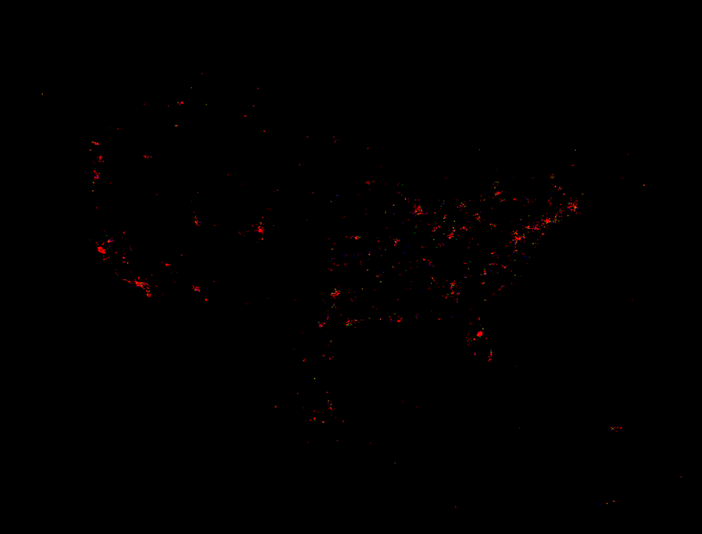
Once Nick had ranked the Pokemon from most-rare to most-common, I asked him to share with me the 10 most common Pokemon types. These are Pokemon so common that they can be found nearly anywhere at any time. If we were to figure out what influences the locations of these Pokemon, I wagered that it would be more productive to look at ones that were less likely to occur in the first place. In other words, I hypothesized that rarer Pokemon must only appear in areas in which the odds of any Pokemon appearing is higher.For example, in low-chance areas, a pidgey might have a 20% chance to appear, while a charizard would have nearly 0%. In a high-probability area, a pidgey might have an 80% chance to appear, while the charizard would be boosted up to maybe a percent. If high and low probability zones exist, then they would be most visible without the "noise" of very common spawns, listed below in tuples of which Pokemon it is and how many data points that were removed from our visualization.
Paras,21352
Magikarp,24542
Venonat,24975
Caterpie,30593
Drowzee,31743
Zubat,31801
Eevee,35620
Spearow,37559
Weedle,86286
Rattata,119542
Pidgey,159265
That left us with only 311360 out of the original 903922 worldwide, and we could focus on the points of data we care about. Notice this time that there are more blue points, green points, and yellow points, showing a better heat-map of the frequency of spawns without the common Pokemon normalizing the data set. I also increased the scale of the map, effectively "zooming in." This helps cut down on the number of red points, as it may show two yellow points instead of one red one, for example. This map is also higher resolution -- feel free to zoom in on it yourself to explore.
This map reveals that there are some states, like Arizona for example, in which there is only one location in the whole state that would garner any rare spawns at all. In Arizona, it appears to be the city of Phoenix -- which also happens to have the highest population in the area, reinforcing the idea that cellphone density is a key determining factor on when things appear, even if it is not yet proven to influence what appears.
In the below gif, we begin with our original data set, and filter out more common species like pidgey, and continuing filtering out more species each frame, until the final frame which contains only the rarest.
Conclusion:
With this visualization, we prove that the nearly all rare spawns happen in population dense areas. As we filter out the more common species, the data retracts further and further into cities. This proves that not only do more spawns happen there, but rarer ones. As we further analyze the data, we will test more claims as to what influences the spawnrate and kinds of Pokemon appear -- our next target being, "Does the weather influence the type of Pokemon that appear?" Overall, this has been a successful first step at gathering, visualizing, and analyzing our Big Data.


Comments